Sparse Autoencoders for More Interpretable RLHF

December 12, 2023

By Laker Newhouse and Naomi Bashkansky

Introduction

Understanding how machine learning models arrive at the answers they do, known as machine learning interpretability, is becoming increasingly important as models are deployed more widely and in high-stakes scenarios. Without interpretability, models may exhibit bias, toxicity, hallucinations, dishonesty, or malice, without their users or their creators knowing. But machine learning models are notoriously difficult to interpret. Adding to the challenge, the most widely used method for aligning language models with human preferences, RLHF (Reinforcement Learning from Human Feedback), impacts model cognition in ways that researchers do not understand. In this work, inspired by recent advances in sparse autoencoders from Anthropic, we investigate how sparse autoencoders can help to interpret large language models. We contribute a novel, more interpretable form of fine-tuning that only learns parameters related to interpretable features of the sparse autoencoder.

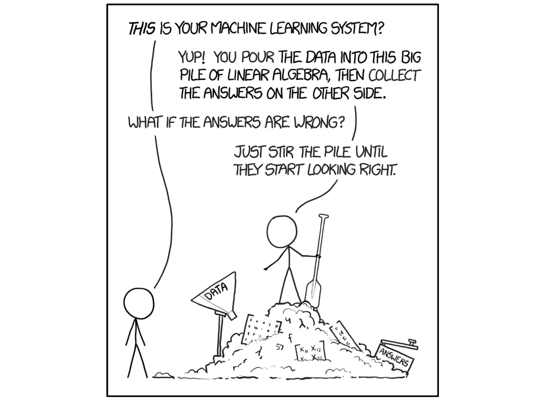
Machine learning practitioners often cannot interpret the models they build (xkcd #1838).

Related Work

Research on interpreting machine learning models falls broadly under one of two areas: representation-based interpretability (top-down) and mechanistic interpretability (bottom-up).

Representation-based interpretability seeks to map out meaningful directions in the representation space of models. For example, Li et al. (Li 2023) found a direction in one model that causally corresponds to truthfulness. Subsequent work by Zou et al. (Zou 2023) borrows from neuroscience methods to find directions for hallucination, honesty, power, and morality, in addition to several others. But directions in representation space can prove brittle. As Marks et al. (Marks 2023) found, truthfulness directions for the same model can vary across datasets. Moreover, current methods for extracting representation space directions largely rely on probing (Belinkov 2022) and the linearity hypothesis (Elhage 2022), but models may have an incentive to store some information in nonlinear ways. For example, Gurnee et al. (Gurnee 2023) showed that language models represent time and space using internal world models; for a world model to store physical scales ranging from the size of the sun to the size of an electron, it may prefer a logarithmic representation.

Mechanistic interpretability, unlike representation engineering, studies individual neurons, layers, and circuits, seeking to map out model reasoning at a granular level. One challenge is that individual neurons often fire in response to many unrelated features, a phenomenon known as polysemanticity. For example, Olah et al. (Olah 2020) found polysemantic neurons in vision models, including one that fires on both cat legs and car fronts. Olah et al. hypothesized that polysemanticity arises due to superposition, which is when the model attempts to learn more features than it has dimensions. Subsequent work investigated superposition in toy models, suggesting paths toward disentangling superposition in real models (Elhage 2022). Superposition is relevant for language models because the real world has billions of features that a model could learn (names, places, facts, etc.), while highly deployed models have many fewer hidden dimensions, such as 12,288 for GPT-3 (Brown 2020).

Recently, Sharkey et al. (Sharkey 2022) proposed using sparse autoencoders to pull features out of superposition. In an interim research report, the team describes inserting a sparse autoencoder, which expands dimensionality, into the residual stream of a transformer layer. In a follow-up work, Cunningham et al. (Cunningham 2023) found that sparse autoencoders learn highly interpretable features in language models. In a study on one-layer transformers, Anthropic provided further evidence that sparse autoencoders can tease interpretable features out of superposition (Bricken 2023). Although interest in sparse autoencoders in machine learning is relatively recent, sparse autoencoders have been studied in neuroscience for many decades under the name of expansion recoding (Albus 1971).

Researchers have begun to apply sparse autoencoders to other interpretability problems. For example, Marks et al. (Marks 2023) investigated whether models on which we perform RLHF internalize the reward signal. To do so, Marks compared sparse autoencoders trained on the base model with sparse autoencoders trained on the fine-tuned model. But, to our knowledge, while others have used sparse autoencoders to probe the effects of fine-tuning, there is no prior research on using sparse autoencoders to define a more interpretable form of fine-tuning. We propose a new form of fine-tuning in which the learnable parameters are related to the interpretable features of the sparse autoencoder.

Background

An autoencoder is an architecture for reproducing input data, with a dimensionality bottleneck. Let $d_\text{model}$ denote the dimension of the residual stream in a transformer. Let $d_\text{auto}$ denote the dimensionality of the autoencoder. To enforce the dimensionality bottleneck, we require $d_\text{model} > d_\text{auto}$. The diagram below depicts an autoencoder.

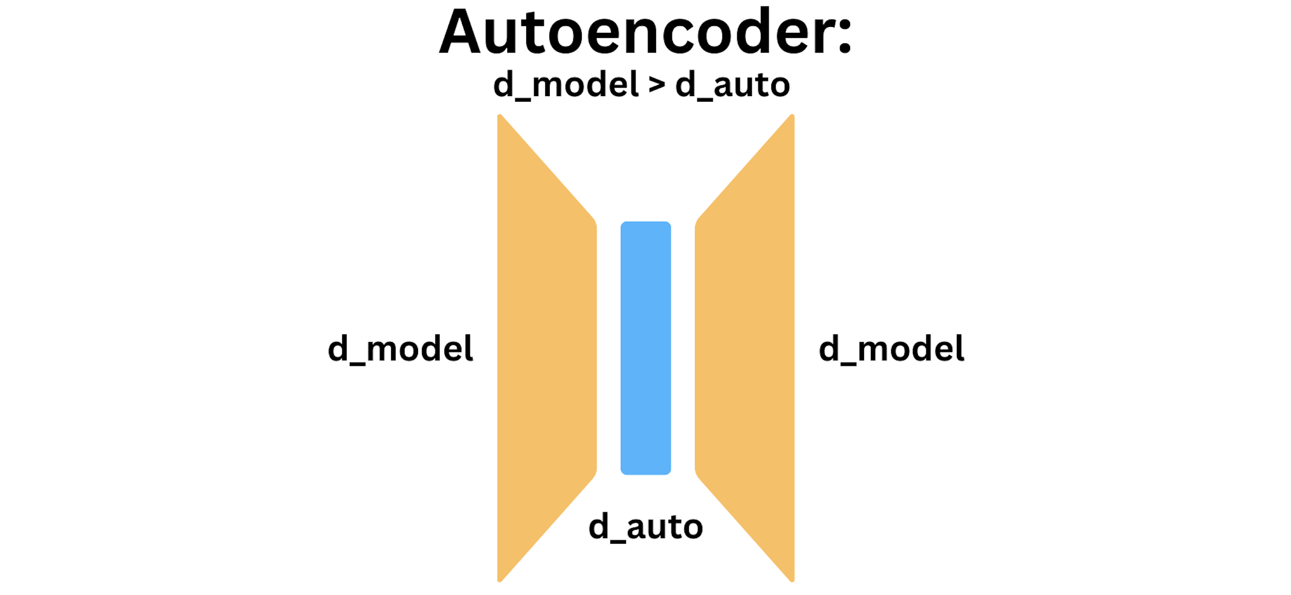
An autoencoder is trained to reproduce its input, subject to a dimensionality bottleneck.

A sparse autoencoder relies on a different kind of bottleneck, called sparsity. For a sparse autoencoder $g \circ f$ that acts on $x \in \mathbb{R}^{d_\text{model}}$ by sending $f(x) \in \mathbb{R}^{d_\text{auto}}$ and $g(f(x)) \in \mathbb{R}^{d_\text{model}}$, the training objective combines MSE loss with an $L^1$ sparsity penalty:

$$\mathcal{L}(x; f, g) = \|x - g(f(x))\|_2^2 + \beta \| f(x) \|_1,$$

where $\beta > 0$ trades off sparsity loss with reconstruction loss. With the sparsity constraint, we can now let $d_\text{auto} > d_\text{model}$ by a factor known as the expansion factor. The diagram below depicts a sparse autoencoder.

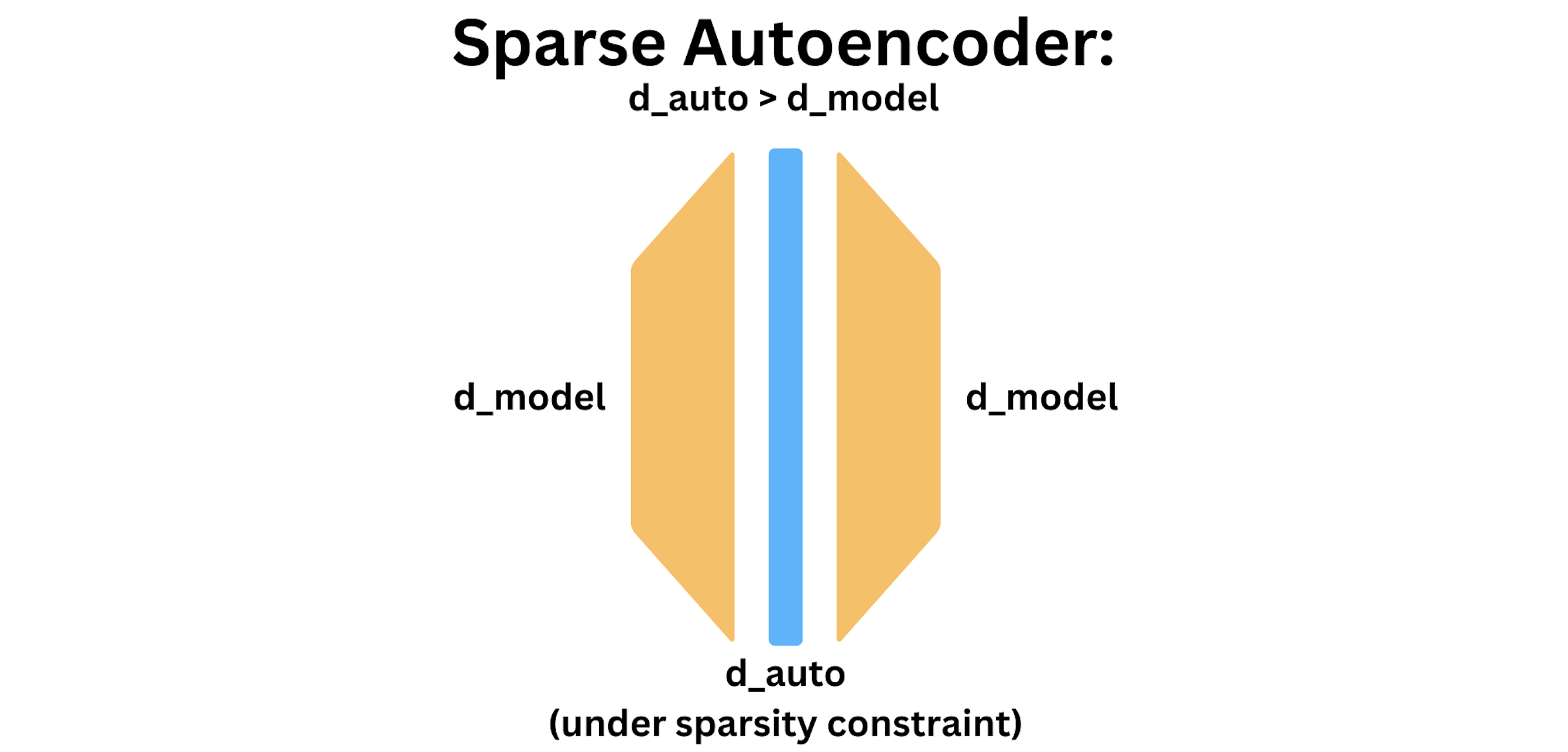
A sparse autoencoder is trained to reproduce its input, subject to an $L^1$ sparsity bottleneck.

Methods

Our main experiment is to insert a sparse autoencoder into a transformer layer, train the sparse autoencoder, and then use the fused model to perform a new, more interpretable form of fine-tuning. We run all experiments on a single A100 GPU through Google Colab Pro+.

Inserting a Sparse Autoencoder in a Transformer

There are three natural places to insert a sparse autoencoder into a transformer:

MLP activations before the nonlinearity
MLP activations before adding back to the residual stream
The residual stream directly

We choose the second option. The upside of operating in the MLP space is that MLP blocks may be in less superposition than the residual stream, given that MLPs may perform more isolated operations on residual stream subspaces. The upside of operating after the MLP projects down to the residual stream dimension is a matter of economy: because $d_\text{model} < d_\text{MLP}$, we can afford a larger expansion factor with the same memory resources.

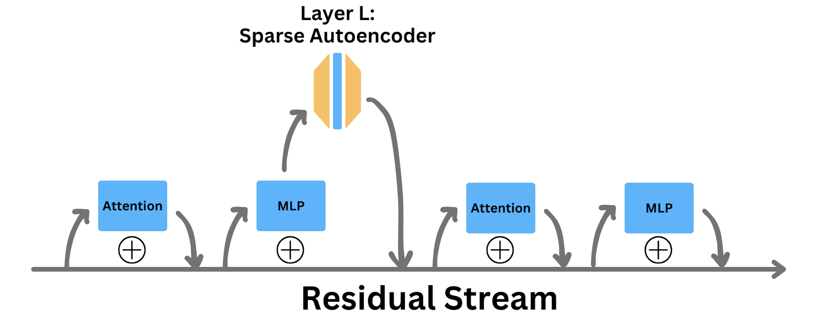
We insert a sparse autoencoder into a transformer after the MLP, but before adding into the residual stream.

How We Train our Sparse Autoencoder

We train our sparse autoencoder to reproduce MLP-post activations in layer one of Pythia 6.9B (deduplicated). To create a dataset of activations for training, we stream in text from an open-source replication of WebText, the dataset used to train GPT-2. For each batch of text, we collect Pythia 6.9B's MLP-post activations at layer one and use these activations as training data for the sparse autoencoder.

Concretely, our sparse autoencoder has four learnable parameters: $W_\text{enc}$, $W_\text{dec}$, $b_\text{enc}$, and $b_\text{dec}$. The second bias $b_\text{dec}$ is used to center the input. The sparse autoencoder encodes, applies a nonlinearity, and decodes its input $x$ as follows:

$$\text{SAE}(x) = \text{ReLU}((x - b_\text{dec}) W_\text{enc} + b_\text{enc}) W_\text{dec} + b_\text{dec}.$$

We constrain the rows of $W_\text{dec}$ to have unit norm by renormalizing after each optimizer step. Another approach to constrain the rows is to remove gradient information parallel to the feature vectors before each optimizer step, and also renormalize the rows. Although we did not implement it, Anthropic found that that the second approach slightly reduces loss (Bricken 2023).

We use an expansion factor of $4$, meaning $d_\text{auto} = 16384$. When training, we use batch size $8$, learning rate $10^{-4}$, and default $\beta_1 = 0.9, \beta_2 = 0.999$ for the Adam optimizer. Because Pythia 6.9B's context length is $128$ tokens, each training step includes activations from $1024$ tokens. We save checkpoints every $20000$ steps ($20.48$ million tokens).

One subtlety in training is that the sparsity constraint can eventually cause some autoencoder neurons to never activate. How to best handle these so-called dead neurons is an open question. We follow Anthropic in resampling dead neurons to new values (Bricken 2023). Because resampling can cause instability during training, we resample only every 10000 training steps. At that point, we say a sparse autoencoder neuron is dead if it has not activated in any of the last 5000 training steps. In an attempt to improve autoencoder performance, Anthropic resampled dead neurons to the feature directions in which the sparse autoencoder performed worst. For simplicity, we resample dead neurons by setting their corresponding rows of $W_\text{enc}$ and $W_\text{dec}$ to Kaiming uniform random vectors. We reset dead biases to zero.

Fine-Tuning

We fine-tune Pythia 70M with our sparse autoencoder inserted in layer one. Instead of adjusting weights everywhere in the network, we constrain fine-tuning to adjust only a small set of interpretable parameters within the sparse autoencoder. In particular, we learn two vectors of dimension $d_\text{auto}$: a coefficient vector $c$ and a bias vector $d$. Just prior to applying $\text{ReLU}$ in the sparse autoencoder, we scale the activations by $c$ and translate them by $d$.

For our fine-tuning experiments, the sparse autoencoder we use is trained on Pythia 70M Chess (a variant fine-tuned on a chess dataset). We insert this sparse autoencoder into the base Pythia 70M, define new learnable parameters $c$ and $d$ as above, and freeze the gradients on every weight in the fused model except the new learnable parameters. We fine-tune on a small dataset of arithmetic questions (EleutherAI/arithmetic). One training example is shown below:

$$\text{Question: What is }(2 * 7) + 2\text{? Answer:}$$

We train with batch size $8$, learning rate $10^{-3}$, and weight decay $10^{-2}$ using the AdamW optimizer (Loshchilov 2018) over $10$ epochs with $200$ steps per epoch. The figure below shows the training loss as we fine-tune.

Results

Our results come in two parts: an exploration of our trained sparse autoencoder on Pythia 6.9B and an analysis of fine-tuning using a smaller sparse autoencoder on Pythia 70M.

Exploring a Sparse Autoencoder

When inserted into Pythia 6.9B at layer one, our sparse autoencoder achieves a loss of $3.201$ (zero-ablation degrades loss to $3.227$) on the held-out dataset WikiText-103, consisting of over 100M tokens from Good and Featured articles on Wikipedia. Pythia 6.9B's baseline loss is $3.193$. Notably, the sparse autoencoder outperforms a zero-ablation of the layer, demonstrating that it learned features that are useful for reconstruction.

As expected, if the sparse autoencoder is inserted into a layer it was not trained for, performance collapses. For example, if inserted at layer $31$ of Pythia 6.9B, the loss becomes $12.586$. Below is a figure showing the additional loss from inserting the sparse autoencoder at the first eight layers of Pythia 6.9B.

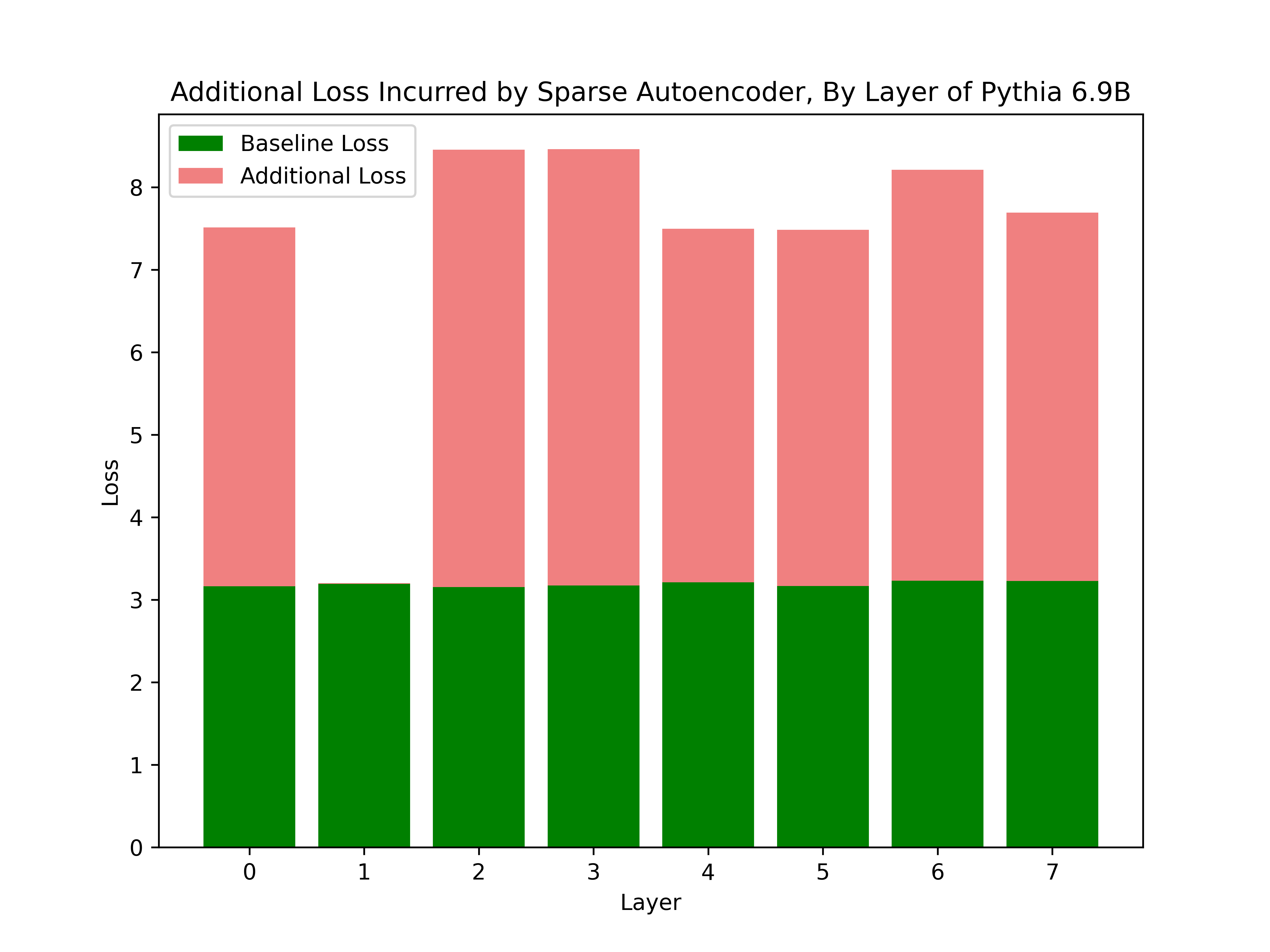
The sparse autoencoder preserves model performance in layer 1, the layer it was trained for. The green bar is loss on WikiText-103 of Pythia 6.9B on 5 random batches. The red bar is the additional loss incurred if the sparse autoencoder is inserted after the MLP at a given layer. The first eight layers are shown.

For more details on the training run, four figures demonstrating the sparsity, $L^1$ coefficient, $L^1$ loss, and reconstruction loss of our sparse autoencoder during training are shown below. After training on the first five million tokens, we automatically begin to adjust the $L^1$ coefficient $\beta$ until we reach the desired sparsity of $1\%$. By the end, our sparse autoencoder stabilizes at a sparsity of $100$, which means that only $0.5\%$ of sparse autoencoder features activate on a given token.

Sparsity across the training run on Pythia 6.9B. On a given batch, sparsity is recorded as the average number of sparse autoencoder features that activate on the batch's $1024$ tokens. Our sparse autoencoder stabilizes at a sparsity of around $100$, or $0.5\%$ of its hidden dimension.

The $\beta$ coefficient in $L_1$ loss across the training run on Pythia 6.9B. After training on five million tokens, we begin to adjust the coefficient until the sparse autoencoder reaches its target sparsity of $1\%$.

The $L^1$ loss of the sparse autoencoder across the training run on Pythia 6.9B. The $L^1$ loss initially rises while the $L^1$ coefficient is adjusted, then falls once the target sparsity is reached as the sparse autoencoder learns a more compact representation.

The reconstruction loss of the sparse autoencoder across the training run on Pythia 6.9B. Reconstruction loss initially rises while the $L^1$ coefficient is adjusted, due to the tradeoff between reconstruction and sparsity. Once the $L^1$ coefficient stabilizes, reconstruction loss slowly falls as the sparse autoencoder learns a more effective representation.

We find that our sparse autoencoder learned several interpretable features. For example, the second most frequently activating feature (feature index 11928) activates strongly on the token “·the”.

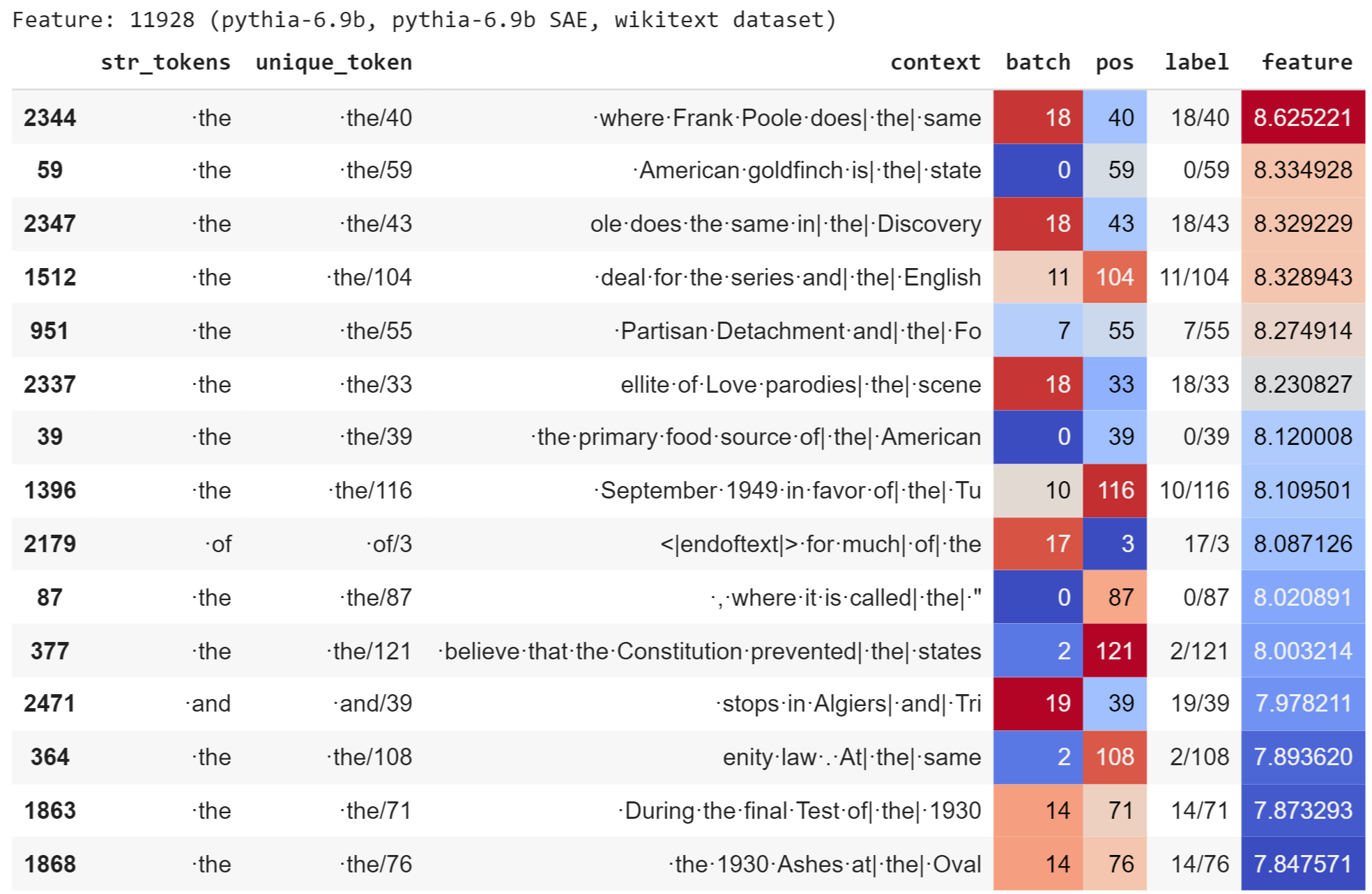
The second most frequent feature (feature index $11928$) in the Pythia 6.9B sparse autoencoder activates on the token "·the". Relevant table columns are $\text{str\_tokens}$ (the token that activates the feature), $\text{context}$ (surrounding tokens in the sentence), and $\text{feature}$ (the raw feature activation in the sparse autoencoder, sorted in descending order). We include the top 15 examples. The feature activates once on “·of” and “·and”, but it activates most on the token “·the”. (Credit: the visualization code for the table is due to Neel Nanda in his open-source replication of Anthropic's sparse autoencoder work.

In addition, we found a surprising correlation between dead features. In particular, almost all dead features point in similar directions, as indicated by a high cosine similarity. In comparison, features that are not dead have a cosine similarity that is much closer to centered at zero. If dead features were drawn from the same distribution as non-dead features, we would expect cosine similarities closer to zero.

The plot above shows the cosine similarity of dead features (red) and non-dead features (blue). Here, a feature is counted as dead if it activates nowhere on WikiText-103-v1. The cosine similarity is calculated compared to the average dead feature. (Credit: the visualization code for cosine similarity is due to Neel Nanda in his open-source replication of Anthropic's sparse autoencoder work.

Fine-Tuning with a Sparse Autoencoder

We fine-tune Pythia 70M on arithmetic data by adjusting only a coefficient and bias vector within the sparse autoencoder space.

On layer $4$, we observe an unexpected lowering of loss from $6.449$ for the base model to $6.270$ after inserting the sparse autoencoder. Once fine-tuning the sparse autoencoder on arithmetic, loss remains constant at $6.270$. We believe that the fine-tuning may perform better when we experiment on a larger model such as Pythia 6.9B.

Although the loss does not fall, several features that our interpretable fine-tuning adjusts are interpretable. For example, the feature that is scaled up the most activates on colons (feature index $1338$). Because colons appear twice in every line of the arithmetic data, it makes sense that the fine-tuned model would like to more readibly predict colons. The figure below shows the top activations of feature $1338$ on the arithmetic dataset before and after fine-tuning. After fine-tuning, the feature activates slightly more strongly in all cases.

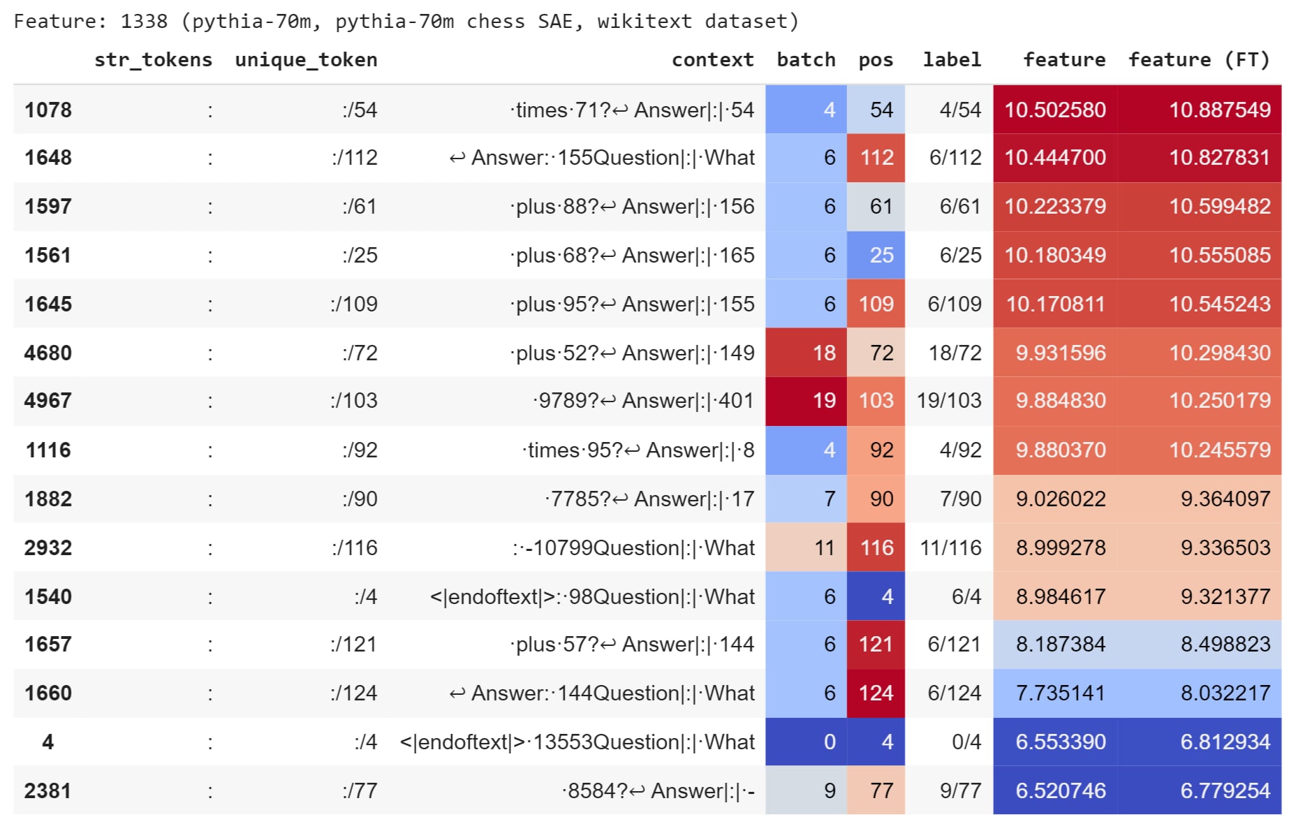
The table above shows the arithmetic dataset tokens on which feature $1338$ most strongly activates, before fine-tuning in the column $\text{feature}$ and after fine-tuning in the column \(\text{feature (FT)}. In all cases, the feature activates slightly more after fine-tuning.

The feature that is most inhibited (feature index $619$) activates on newlines. We hypothesize that the sparse autoencoder learns to avoid newlines because, in the chess dataset for which it was trained, newlines are always followed by “Score: ”, indicating the start of a new game. But in the arithmetic dataset, newlines are always followed by “Answer: ”. Therefore, the model wants to inhibit this unhelpful feature. The discrepancy is a difference in datasets. To rigorously verify this hypothesis, we could compute direct logit attributions from feature $619$ to check whether it contributes to the “Answer” token. Either way, the inhibition above demonstrates that our fine-tuning procedure can detect and modify unhelpful features in the sparse autoencoder.

For a broader view of the dynamics of our interpretable fine-tuning, the two figures below show the learned scale and bias terms across every feature in the sparse autoencoder space (where $d_\text{auto} = 2048$), sorted in ascending order. We observe that the majority of features are largely unaffected, but a few features at the tails are significantly enhanced or inhibited.

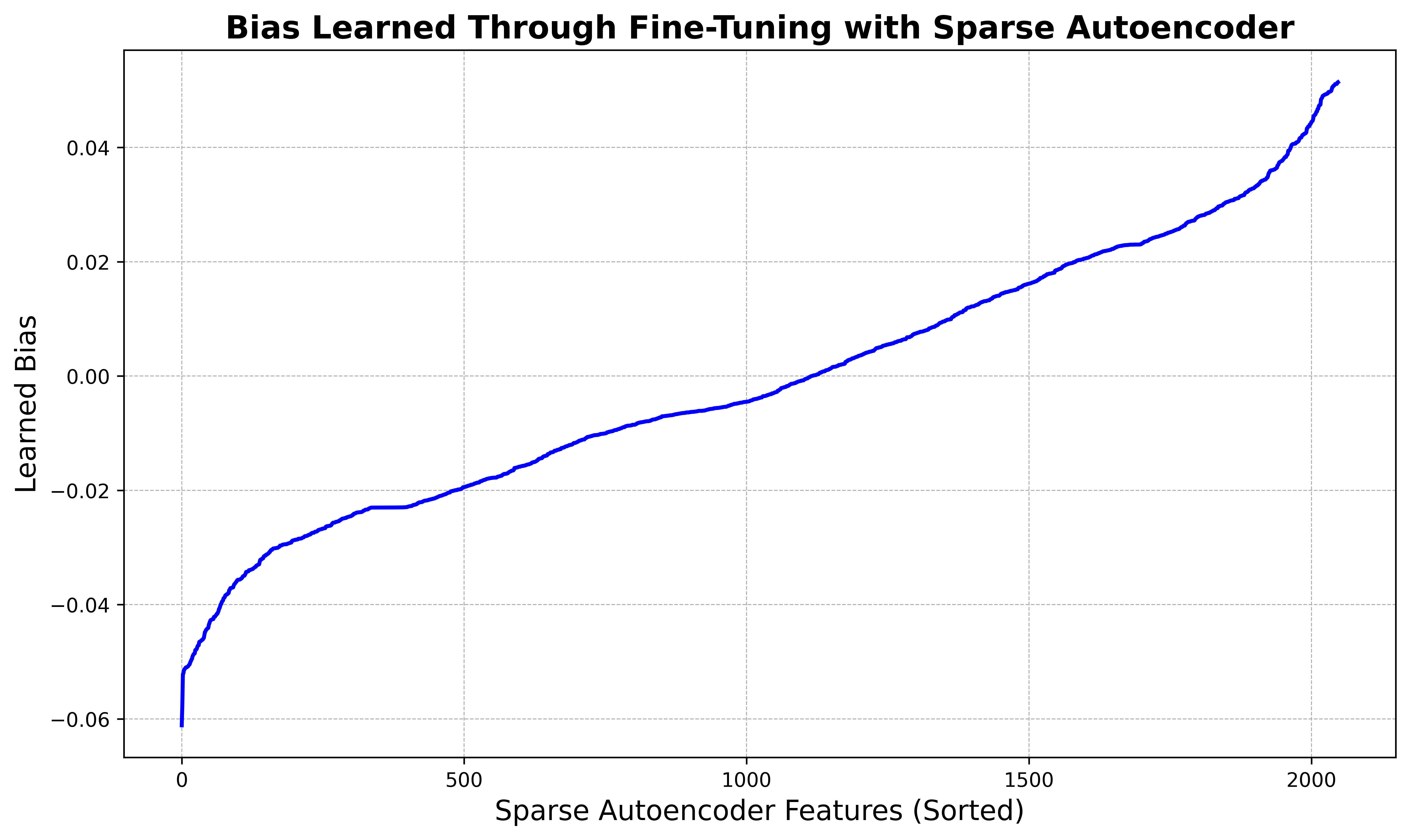
The learned bias in the sparse autoencoder space inhibits approximately half of features while enhancing the other half. The x-axis is sorted so that the feature index runs in ascending order of the learned bias.

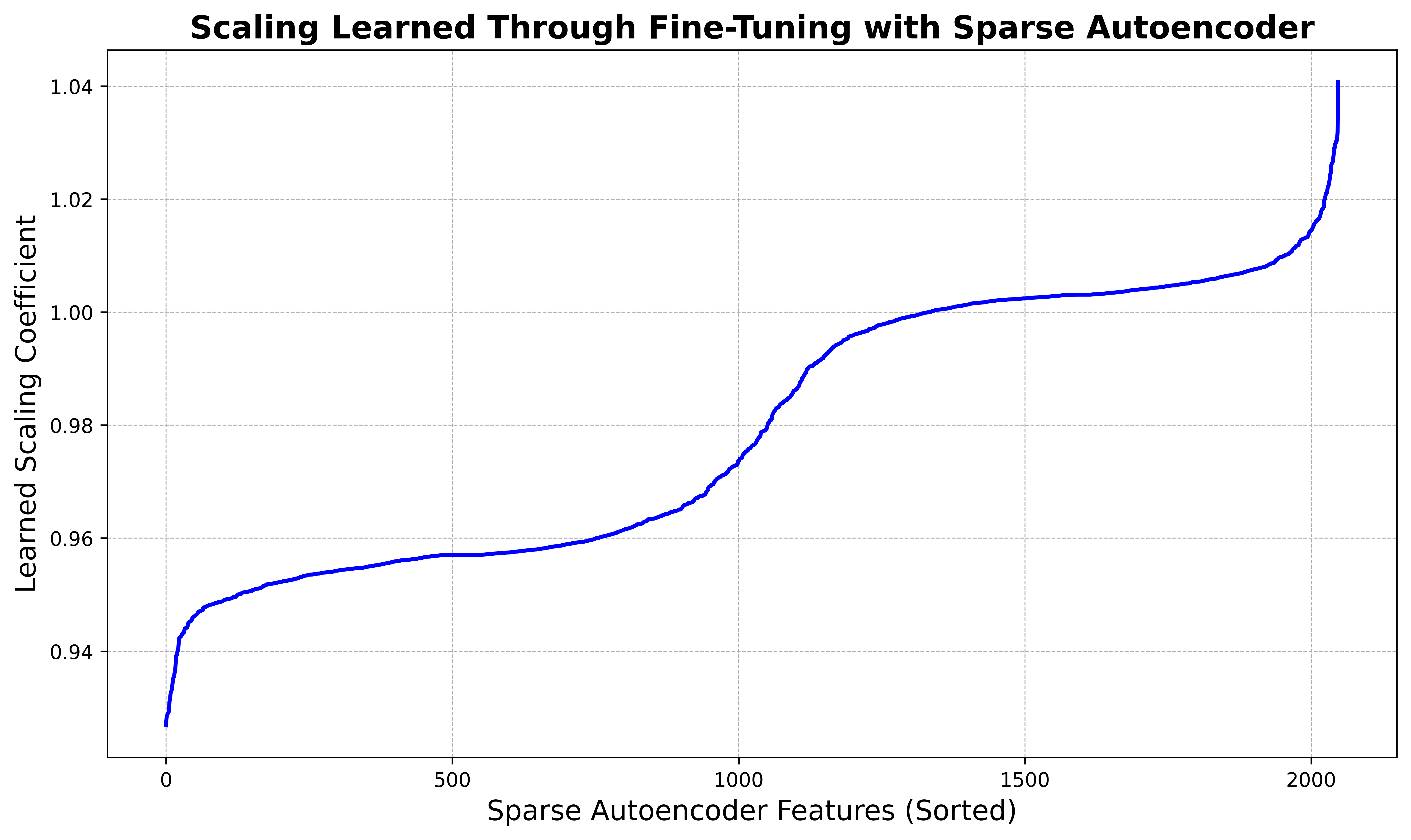
The learned scaling coefficient in the sparse autoencoder space significantly inhibits a small number of features while significantly enhancing several others. We also observe that a majority of features ($2/3$) are inhibited, compared to a smaller number enhanced. The x-axis is sorted so that the feature index runs in ascending order of the learned scaling.

Discussion

One limitation of our fine-tuning experiments is that Pythia 70M is a small model for which there are fewer interpretable features. In addition, we inserted into Pythia 70M a sparse autoencoder trained to reconstruct activations in Pythia 70M Chess. Nonetheless, our fine-tuning results are promising. The majority of features are not significantly affected, but a few features at the tails are either significantly enhanced or inhibited. We found it fruitful to interpret these outlier features first, as they are a starting point for finding which sparse autoencoder features matter most for the fine-tuning dataset.

When training a sparse autoencoder on Pythia 6.9B, we were successful in learning interpretable features, such as the "the" feature. But we remain uncertain of the best way to train a sparse autoencoder, especially how to resample dead features. However, one implication of our work is that research on sparse autoencoders is accessible to a wide array of researchers. We believe a systematic study of training techniques for sparse autoencoders could benefit the field.

Conclusion

Our work indicates that sparse autoencoders are a promising tool for machine learning interpretability. By inserting sparse autoencoders into transformer language models, we investigate how a novel form of fine-tuning can provide insight into changes in model behavior after fine-tuning. We find that our fine-tuning successfully modifies interpretable features in the sparse autoencoder space. Given the rapid adoption of powerful, fine-tuned language models across industries, we believe our method for interpretable fine-tuning is an important direction to continue to explore as researchers seek to understand how fine-tuning affects model cognition. Although our current work is limited because we only fine-tune Pythia 70M, future work can scale up model size, compute resources, and the number of tokens used to train the sparse autoencoder. Additionally, future work can extend from direct fine-tuning to investigating the effects of RLHF performed with PPO (Proximal Policy Optimization).

Acknowledgements

We would like to thank Professor Isola, Professor Beery, and Dr. Bernstein for an introduction to fundamental perspectives in deep learning that will stay with us forever; Logan Smith for invaluable early guidance on the questions we could explore related to sparse autoencoders; and the AI Safety Student Team at Harvard (AISST) and MIT AI Alignment (MAIA) for a supportive community of fellow researchers.

Appendix

Our code is available at the following Google Colab notebooks: